How to read an
audio oscilloscope.

By: AudioWrench product team · Published: October 8, 2026 · Last technically reviewed: October 8, 2026

Open the clean sine exercise →

An audio oscilloscope shows samples against time

The horizontal direction is time; the vertical direction is sample amplitude. This is a short-window view of the actual decoded samples, not a full-song peak envelope and not a frequency spectrum. A smooth repeating signal is easy to inspect. Speech and music often look irregular because several components overlap.

Timebase

Milliseconds per horizontal division. At 1 ms/div, ten divisions span 10 ms. At 5 ms/div, they span 50 ms. Changing timebase changes the inspected window, not the playback speed.

Vertical scale

Normalized amplitude per vertical division. At 0.1/div, eight divisions span 0.8 units, from −0.4 to +0.4 around zero. It changes screen magnification, not the recording’s gain.

Trigger

A chosen amplitude crossing stabilizes a repeating waveform. Rising means below-to-above; falling means above-to-below. AudioWrench places the matched crossing near 25% of screen width. With no crossing at that level, the scope uses an untriggered window.

Cursors

Two sample positions, A and B, report time and amplitude differences. They are independent of the automatic period estimate. Clicking the screen places them; a third click starts a fresh pair.

Digital amplitudes are not calibrated volts, microphone sensitivity or sound-pressure level. The familiar −1 to +1 range is a digital convention; floating-point audio can exceed it. A tall trace is not a loudness reading in LUFS, and a short-window RMS value is not integrated loudness.

Set up a reference, step by step

1. Choose a learning example. Open a linked exercise below, or choose it under Next demo or learning example. The link only selects an option: it does not generate a signal, play audio or request your microphone.
2. Press Generate learning example. This replaces the current source with five seconds of locally generated stereo samples at the browser audio context’s sample rate. The stopped frame is immediately readable. The original 440 Hz stereo demo remains a separate option.
3. Read the actual settings. Learning examples start at 1 ms/div, 0.1/div, rising trigger at zero, and Mix. Compare the measured readouts with the expected relationship, not with a decorative drawing.
4. Measure and save. Place cursors, try another scale or channel, then use Freeze display and Download PNG. Press Start only if you want playback. Freeze holds the display while playback can continue; Stop stops playback too.

1. Clean sine: measure a period, then calculate frequency

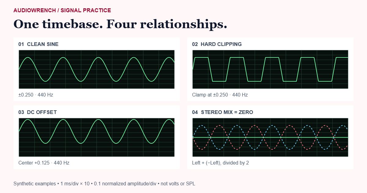
This reference is 0.25 × sin(2π × 440 × t) in both channels. At 1 ms/div you see about 4.4 cycles across the screen. The peaks approach +0.250 and −0.250, so peak-to-peak is approximately 0.500. Changing from Mix to Left or Right should not alter it.

Put cursor A on one rising crossing of the zero line and cursor B on the next rising crossing. Use the same phase point in consecutive cycles — measuring from a rising crossing to a falling crossing would give half a period. Read Δ time, then take its reciprocal:

frequency (Hz) = 1000 / Δ time (ms)
1000 / 2.273 ≈ 440 Hz

At 44.1 kHz one sample is about 0.02268 ms; at 48 kHz it is about 0.02083 ms. Cursor positions are snapped to samples, so manual results need not equal the automatic estimate. The automatic readout averages interpolated rising crossings relative to the window mean. It needs several accepted cycles and sufficient signal amplitude; it is not a calibrated frequency counter.

2. Flat tops: distinguish sample clipping from display zoom

This example deliberately amplifies the sine to 0.65 and clamps the samples to ±0.250. Flat sections are now part of the data. Peak-to-peak is still 0.500, but the curve spends more time at its ceiling and floor. That is why equal peak-to-peak values do not mean equal waveform shape or RMS.

Change Vertical scale from 0.1/div to 0.2/div. The curve becomes smaller but the flat tops remain. By contrast, if you magnify the clean sine enough to push it beyond the screen edges, you have only cropped the drawing. Zooming out restores the smooth peaks; the samples were not clipped.

3. DC offset: a shifted center without a bigger peak-to-peak span

This reference adds a constant +0.125 to the clean sine. Its expected range becomes −0.125 to +0.375; peak-to-peak remains 0.500. The curve’s center is above zero even though its oscillating component has not grown. At 0.1/div it fits inside the screen, making the asymmetry easy to see.

Increase Trigger level to +0.12 and retain Rising edge. The control moves in 0.01 steps, so this is close to the sine’s +0.125 center, not an exact center setting. Changing that crossing can reposition the curve but cannot remove the offset. The frequency estimate should remain near 440 Hz because the measurement subtracts the window mean when finding crossings.

4. Silent Mix: two audible channels can cancel

Left is the clean ±0.250 sine. Right is exactly its negative, sample for sample. The selected Mix is an arithmetic average, so the expected result is a flat zero trace:

Mix = (Left + Right) / 2
(x + (−x)) / 2 = 0

No frequency estimate and no zero-crossing trigger are expected for that silent Mix. Choose Left: the sine and approximately 440 Hz should return. Choose Right: the signal remains 440 Hz with opposite polarity. A rising trigger stabilizes each channel on its own rising crossing, so those two separately triggered drawings can look alike. That does not undo the inversion.

The Channel selector changes what the scope displays; it does not convert the playback buffer to mono. Playing this stereo example can still be audible through separate left/right outputs even while the displayed Mix is zero. To hear an actual downmix, export through Stereo to Mono and compare that result.

Move from a reference to your own audio or microphone

Choose audio to decode a supported file locally. WAV, MP3, FLAC and other formats depend on the browser’s codec support. The encoded-file limit is 80 MB, with additional decoded-memory, duration and mono/stereo guards. The scope is not a full-file scanner: file playback moves its short inspection window through the recording, and the display can wrap at the file boundary.

Use microphone requests permission only after you press it. Its samples are inspected without routing the microphone to speakers. Stop closes the active microphone tracks. Echo cancellation, automatic gain and noise processing are requested off, but hardware and browser behavior still affect the input; this does not turn your microphone into a calibrated lab instrument.

Choose a timebase that exposes the question you are asking. A steady tone needs several cycles for a reliable estimate; complex music may have no useful single period. Put the trigger level inside the signal’s actual range. If a stable value disappears on noise or silence, that can be the honest result, not a broken counter.

For a static inspection, Freeze display holds the samples and measurements. On the focused canvas, press 1 and 2 to place cursors, arrows to move the active cursor, Shift+arrow for a larger move, Escape to clear, F to freeze, and Space to start or stop. Download PNG saves the current scope canvas, not the whole web page and not an audio file. Keep a separate note of source name and settings if you need a repeatable comparison.

Oscilloscope, waveform overview or spectrum?

Oscilloscope

Use a short time-domain window for cycle shape, timing, amplitude and known periodic relationships.

Waveform overview

Use Waveform Generator for the whole recording’s peak envelope, broad dynamics and a shareable overview image.

Spectrum over time

Use a spectrogram for how frequency energy changes through a recording. Neither a time-domain curve nor a spectrogram alone measures perceptual quality or identifies every processing artifact.

The examples and their explanations are free. Generated and selected audio are processed in the browser; ordinary page assets follow the privacy notice. No account or microphone is needed to complete these four exercises.

Open the audio oscilloscope →

Related tools